Causal Modeling: Multiplying Data With Mechanism

The competitive edge in drug development is whatever lets you extract more signal from the same evidence. A causal model is the analytical layer that combines observed data with mechanistic knowledge about the underlying biology. That combination is often what gives better predictions than either alone.

A correlational model — a regression, a classifier, most of standard machine learning — encodes statistical associations between variables. A causal model encodes a hypothesis about the mechanism that generates the data: which variable depends on which, in what direction, and how. The data is used to calibrate parameters, test predictions, and reject the hypothesis when it fails.

Causal modeling is not a single technique. The mathematical representation follows from the structure of the question — whether the biology has feedback loops, whether time matters, what counts as an intervention, and what measurements are available. The right framework is whichever one matches the structure of the problem.

When the mechanism can be written as a one-way chain — upstream factors drive a target, the target drives an outcome, no downstream variable loops back to alter an upstream one — a directed acyclic graph (DAG) is the natural fit (Pearl, Causality, 2009). The moment time matters — drug clearance, autoregulation, a downstream product inhibiting an upstream pathway — the problem becomes fundamentally dynamic. While such systems can still be represented with time-indexed DAGs, ordinary differential equations often provide a more natural description because they explicitly model how system state evolves over time. Quantitative systems pharmacology and PK/PD models live here, and also higher level systems biology models of diseases (Alon, System's medicine, 2024). 

What these causal frameworks share is that the structure represents assumptions about mechanism; the data calibrates and tests the model; and the model can be interrogated under hypothetical interventions. In Part 2 of this blog we will show an example — a single-arm trial in advanced bladder cancer — there are no feedback loops in the biology we need to capture, and the data is cross-sectional rather than time-resolved. A DAG is the right tool.

What a DAG-based causal model looks like

In a probabilistic causal model, the graph is a network representing the hypothesis regarding the underlying mechanism. Each node is a random variable; the edges encode which variable conditions which. Observing a value at one node propagates information through the graph: the conditional distribution at every other node updates to reflect what you now know.For example, the nodes can represent treatment, the biological target it acts on, the downstream outcome, plus the upstream patient factors that shape both target and outcome (patient biology, tumor characteristics, prognostic markers). The arrows (directed edges) are the causal assumptions: which variable depends on which, and how (e.g., linearly, nonlinearly). Every arrow is drawn from literature and basic experiments — not estimated from the trial data.

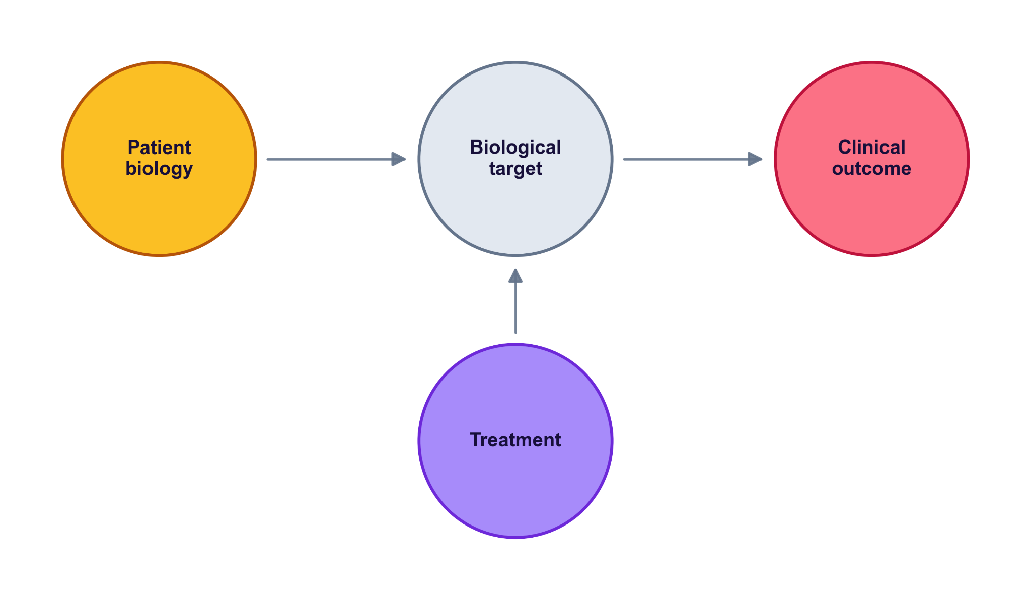
The figure above is a scaffold. In a real model, the arrows reflect what’s actually known about the biology, and the nodes get filled in with specifics — a particular biomarker, a measured endpoint, a pathway intermediate. The shape stays; the contents become specific to the question at hand. In Part 2's worked example — atezolizumab in advanced bladder cancer — the treatment is the drug, the target is PD-L1 (a ligand on tumor cells), the outcome is tumor growth, and the upstream factors are immune phenotype and tumor mutation burden. The arrows encode the mechanism: the drug blocks PD-L1 to release T cells against the tumour. We unpack each piece there.

That structure is what lets the model answer questions the data on its own can’t (“what if questions”):

•      What would the same patient have looked like untreated? — carry them through the graph with the treatment node turned off.

•      What happens in a different subgroup? — shift the upstream-factor distribution.

•      What if the dose were different? — change the treatment-to-target arrow.

Hidden assumptions are worse than wrong ones

The trade-off is stated up front: every assumption is now explicit and falsifiable. That is the property that makes the framework worth the work.

A causal model puts each assumption on a named arrow. If an arrow is wrong, the model is wrong in a way you can locate, examine, and replace. *"The drug acts on target X"* is an arrow. *"Mutation burden modulates that effect"* is an arrow. *"The upstream patient factor is independent of treatment assignment"* is the *absence* of an arrow — and that absence is just as falsifiable as the arrows that are drawn.

Two practical consequences follow. First, when results look surprising, debugging becomes a structural exercise rather than a fishing expedition: enumerate the arrows the result depends on, find the one that doesn't survive scrutiny, replace it. Second, the model can be argued with. A reviewer who disagrees with the analysis can point to a specific arrow and explain why they would draw it differently — and the disagreement becomes resolvable rather than rhetorical. Hidden assumptions don't have either property: nothing in a correlational model invites that kind of conversation, because the load-bearing claims are not named.

A live model, not a black box

A causal model’s value isn’t in any single version — it’s in the discipline of writing the assumptions down and updating them as evidence accumulates. A new preclinical result, a new biomarker, a new trial readout: each is a chance to revise an arrow, add a node, or retire one that didn’t earn its place. The most informative analysis is usually the comparison between successive versions of the model, not the defence of a single static one.

The traffic runs both ways. Once every assumption is laid out in one logical structure, the model also points to where the next experiments should go. It can reveal that a biomarker you treated as secondary is more informative than the data first suggested, or that what looks like one disease is actually two subgroups manifesting through different pathways. And it helps prioritise experiments by where the assumptions are weakest — confirming a shaky arrow is as valuable as overturning it. 

A simple model is what makes iterative refinement and experimental prioritization possible. Keep the model simple and you can react to new biology quickly. Bury it in nuisance parameters and you can’t — the model becomes its own bottleneck. In structuring a model, it is just as important to consider which interactions to leave out. Every model is the draft of the next model.

The trade-off is stated up front: every assumption is now explicit and falsifiable. That is the property that makes the framework worth the work.
A causal model puts each assumption on a named arrow. If an arrow is wrong, the model is wrong in a way you can locate, examine, and replace. *"The drug acts on target X"* is an arrow. *"Mutation burden modulates that effect"* is an arrow. *"The upstream patient factor is independent of treatment assignment"* is the *absence* of an arrow — and that absence is just as falsifiable as the arrows that are drawn.
Two practical consequences follow. First, when results look surprising, debugging becomes a structural exercise rather than a fishing expedition: enumerate the arrows the result depends on, find the one that doesn't survive scrutiny, replace it. Second, the model can be argued with. A reviewer who disagrees with the analysis can point to a specific arrow and explain why they would draw it differently — and the disagreement becomes resolvable rather than rhetorical. Hidden assumptions don't have either property: nothing in a correlational model invites that kind of conversation, because the load-bearing claims are not named.

When mechanism stops being optional

In data-rich settings you can let correlations speak for themselves and still land somewhere sensible. In clinical development you usually can’t. Sample sizes are small. The biology is characterised from years of preclinical work. Single-arm Phase 2 designs — increasingly common in oncology and rare disease — give you no measured control to lean on.

As data thins, causal structure moves from useful to necessary. Every defensible assumption brought in from outside the dataset is worth more than it would be at scale — because the dataset can no longer carry the question on its own.

The point isn’t that mechanism replaces evidence — only an experiment delivers that. The point is that the analysis you bring to the evidence determines how much of your existing knowledge you actually get to use.

In the next post we apply this scaffold to a real single-arm Phase 2 trial in advanced bladder cancer — and show what changes when the model gives us the control arm the trial didn’t measure.

When the data is too thin to answer the question on its own, a causal model is what brings the rest of what you know — the biology — back into the prediction. And it gets stronger every time you update it.

‍