Oncology Phase 2 studies are often small, split across biomarker-defined subgroups, and frequently single-arm, leaving a fragmented view of disease biology and treatment response. To make sense of that fragmentation, we need a way to connect patient measurements, biological mechanisms, treatment, and outcomes. Causal models provide a framework for connecting data to biological mechanisms and exploring why patients respond differently, how outcomes vary across cohorts, and what might happen under alternative biological or treatment conditions. That missing layer can fundamentally change how the results are interpreted.

Why a model, and why causal

To make this concrete, we focus on a case study of IMvigor210, a real single-arm Phase 2 trial of atezolizumab in metastatic urothelial carcinoma, an advanced form of bladder cancer. Atezolizumab is an immunotherapy that helps T cells attack tumors by blocking PD-L1, a signal tumors can use to dampen the immune response.

All patients in the trial received atezolizumab, so the study does not directly show what would have happened without treatment. What makes it useful for this example is that it collected rich pre-treatment biomarker data, giving us a detailed snapshot of each patient’s tumor biology before therapy. We use those measurements to calibrate the causal model.

To estimate a treatment effect we would ideally want to compare each patient's outcome under the drug to what would have happened to them without it. The single-arm structure gives us the first; it gives us nothing about the second.

A standard predictive model trained on the trial would not close that gap. A regression of response on baseline biomarkers learns correlations between features and the observed (treated) outcome — it has nothing to say about what those same patients would have looked like untreated, because no untreated patients appear in its training data. A causal model is different: instead of leveraging associations for predictions, it encodes hypotheses about the mechanism that generates the data — which variable depends causally on which. Once the mechanism is laid out, the model can be interrogated under interventions it never observed. For example, one may ask how the same biological system behaves under alternative treatment conditions, including the hypothetical no treatment scenario. Such analyses do not reveal the true counterfactual, but they provide a mechanistically grounded prediction conditional on the assumptions encoded in the model.

Causal models are powerful, but they come with an important caveat. A causal graph alone does not determine a credible counterfactual. The difficulty lies in specifying the quantitative relationships along each edge, validating that the resulting model generates biologically plausible patient profiles and reproduces key patterns in the observed data, and identifying which biological processes are directly affected by treatment. When simulating a counterfactual scenario, for example a control arm, it is not enough to switch a treatment indicator from on to off; one must also account for how treatment changes the parameters governing tumour growth, immune activity, or other downstream processes. Those assumptions must be justified biologically and tested against available evidence.

In the worked example below, we use the model to ask what outcomes might have looked like for the same trial population under a hypothetical no-treatment scenario. The example is intended as an illustration of the process rather than a fully validated virtual control arm. Its purpose is to show how biological knowledge can be encoded into a causal model, calibrated against patient-level data, and then used to explore counterfactual scenarios. In practice, the credibility of any estimated control arm depends on careful model validation and scrutiny of the treatment-dependent assumptions that drive the predictions.

A Probabilistic Graph: How Biology is Encoded in the Model 

Building the model starts before any equations are written. The first step is a focused literature review around the specific causal question: for this drug, in this disease setting, which biological processes are most likely to determine response? The goal is not to include every known feature of tumour immunology. A useful model should be detailed enough to capture the mechanisms that matter for the question, but simple enough that the main assumptions remain visible. 

At the first pass we concentrate on building a scaffold that includes the treatment, treatment target and biological outcomes, and we add details and nodes as needed. In the example below, the treatment is atezolizumab, an anti-PD-L1 checkpoint inhibitor; its target is PD-L1 on the tumour cell surface; the outcome we model is tumour growth C after treatment. 

After identifying the treatment, treatment target and biological outcome, we consider which biological entities are mediators leading from the treatment to the biological outcome, and add them as nodes. Each candidate node is chosen deliberately. Some are included because they are plausible drivers of response; others are included because they are measured in the trial and help anchor the model to data. In our example, the mechanism connecting the treatment to the outcome is the PD-1 / PD-L1 brake: CD8 T-cells can kill tumour cells, but tumours often express PD-L1, which binds PD-1 on T-cells and switches off their killing function. Atezolizumab blocks that interaction and restores T-cell function — but only when a T-cell is present and active.

 
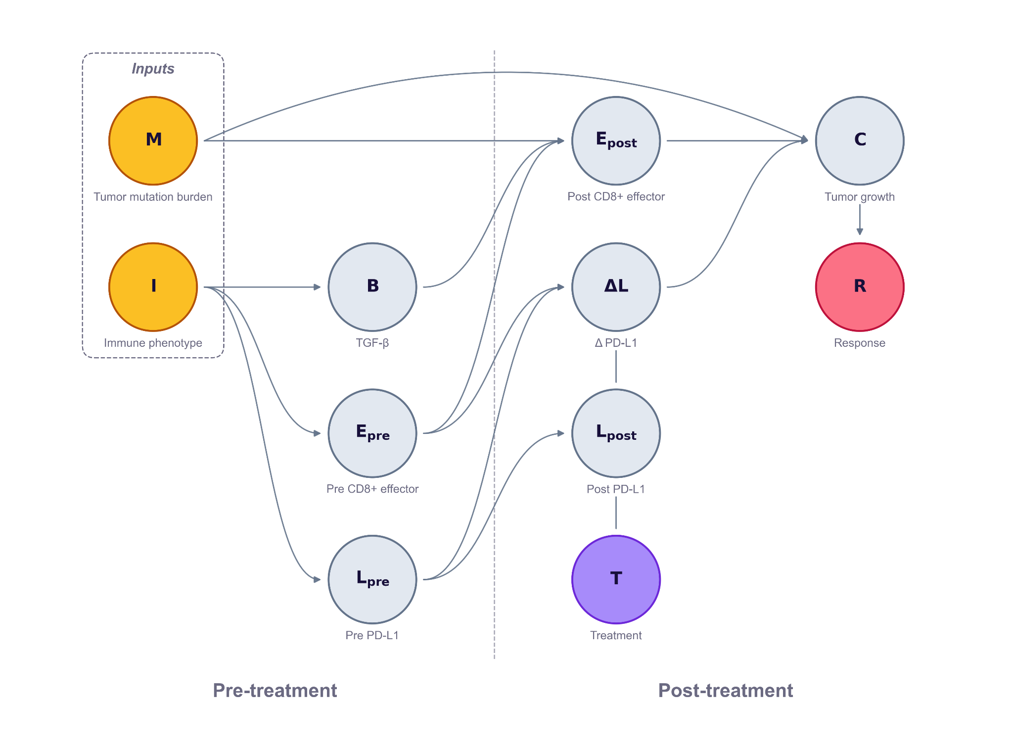
But the same drug against the same target produces very different outcomes patient to patient, depending on the pre-treatment immune state of the tumour. To capture that patient-to-patient variability, the model includes the pre-treatment biomarkers from Mariathasan et al. (Nature 2018) that determines whether PD-L1 blockade reduces tumor growth. CD8 T-effector activity measures whether killer T-cells are present and active to begin with — the drug has nothing to unleash if they're absent. Tumour mutation burden counts how many neoantigens those T-cells might recognise as foreign — more mutations means a more visible tumour. TGF-β signalling can physically exclude T-cells from the tumour by building a stromal barrier — the brake-release doesn't help if T-cells can't reach the cancer cells. PD-L1 expression measures how much brake there is to release in the first place. Mariathasan also groups patients into three immune phenotypes that summarise the spatial pattern of T-cell infiltration: inflamed tumours have CD8 T-cells already inside the tumour, ready to attack, and respond best to checkpoint blockade. Excluded tumours have T-cells trapped outside the tumour by TGF-β-driven stromal barriers, so brake-release doesn't help much. Desert tumours have no T-cell infiltration at all, leaving the drug with nothing to act on.

The mechanism leads us to add two upstream inputs — immune phenotype and tumour mutation burden — which drive three observable pre-treatment markers PD-L1 expression, CD8 score, TGF-β level. These markers then combine with the treatment indicator T to determine post-treatment tumour growth C. The  parameters of the model, such as the strength and direction of each effect, is calibrated against the patient-level biomarker data from IMvigor210 Cohort 2.

When selecting the nodes, each measurement is scrutinized. A biomarker is not automatically the biological process it is meant to represent. PD-L1 staining, CD8 expression, TGF-β signatures, and tumour mutation burden are all operational measurements, produced by specific assays, cutoffs, sampling procedures, and tissue contexts. For each one, the model builder has to ask: does this measurement directly reflect the biological node we care about, or does the experimental procedure introduce another source of variation that should be represented in the graph? In some cases, the assay can be treated as a reasonable proxy. In others, the measurement process itself may warrant an additional edge or node.

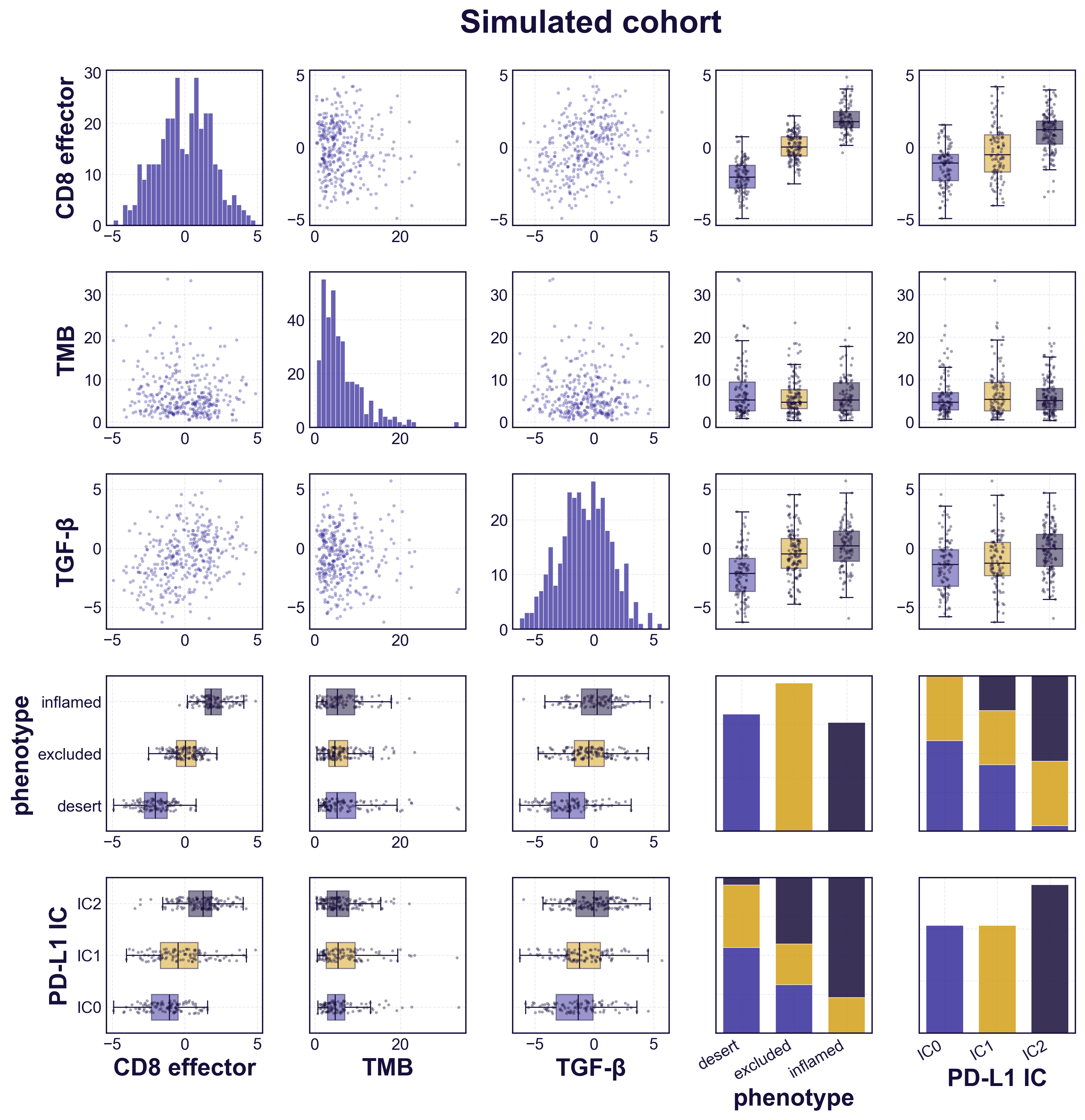
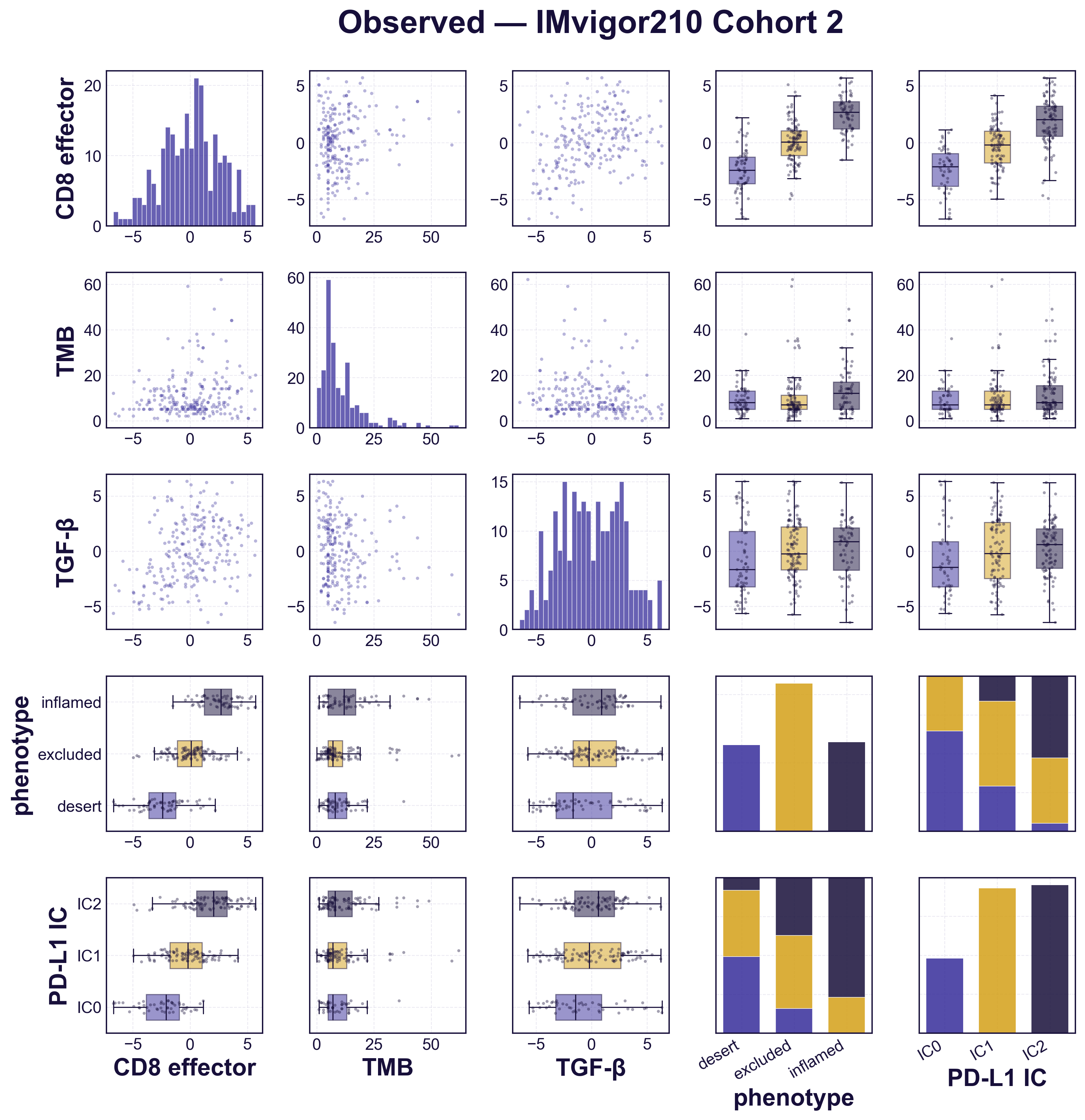
Before using the model to explore counterfactuals, we check that it reproduces the data it was built from. We simulate a cohort the size of the trial population and compare it against the real patients, biomarker by biomarker (figure). The simulated distributions match the observed ones, and each biomarker varies across the three immune phenotypes the way it does in the trial — CD8 activity and PD-L1 rising from desert to inflamed tumours, TGF-β lowest in desert. The simulated cohort is distributed like the real one, confirming the model is faithfully calibrated to the patient-level data before we ask it anything counterfactual.

With the graph in place, the model can be used to explore alternative interventions. The same simulated patient can be propagated through the graph under different treatment assumptions, biological states, or parameter settings. One possible analysis is to compare outcomes under T = 1 and T = 0, generating a model-based estimate of how treatment changes the predicted outcome for that patient. Other analyses might examine the consequences of changing biomarker levels, modifying specific biological pathways, or testing competing mechanistic hypotheses. The goal is not to replace the experiment, but to make the most informed estimate possible about the missing arm when no untreated comparison was actually observed. The quality of that estimate depends on how well the underlying biology is understood, but it allows the comparison to be grounded in mechanism and available data.

Try It Yourself

The figure embeds the simulator. The default cohort matches the empirical biomarker profile of the trial data; the plot shows one possible counterfactual analysis: the distribution of tumour growth `C` for the simulated treated and control arms side by side. The gap between them — in medians, 50% intervals, and response rates — is the model's estimate of the treatment effect for that cohort.

Move the sliders and both arms re-run. Push the cohort towards immune-desert and the gap narrows; towards inflamed and it widens; raise median tumor burden and the treated arm pulls further away. 

The simulated treatment effect is not evidence of efficacy — only an experiment delivers that. What the model offers is the best prediction the available evidence permits, combining patient-level data from past trials with biological mechanisms. This provides more rigorous interpretation than either a model or data can alone. That makes this approach useful for designing follow-up trials, interpreting published response rates, and surfacing the biological assumptions driving the predictions — not for substituting an experiment with a randomized control arm.

The figure above illustrates one possible application. More broadly,  causal models bring biological mechanisms and patient-level data together — carrying knowledge across trials, answering questions the trials themselves never directly asked, and pointing to where the next experiment is most likely to pay off.