Real-World Data Is Noisy. Your Model Has to Know That.

Anyone who has worked with electronic health records knows an unspoken truth: the data is rarely as clean as the questions we ask of it. Notes are typed in a hurry, scales switch between pounds and kilograms, and simple typos are common. When you multiply these small errors by tens of thousands of patients over several years, you are left with a dataset that looks rich but is alarmingly noisy.

For data scientists in pharma and biotech, this is everyday terrain. Finding ways to see through this noise is where some of the most critical work happens.

The Challenge: Tracking Real Progress

In a recent observational study, we wanted to understand how different weight-loss approaches — such as medication, surgery, or lifestyle changes — affected people living with obesity and related conditions like sleep apnea or heart disease. The analysis hinged on a simple question: how much weight did each patient actually lose? If we get that number wrong, every other finding about which treatments impact becomes unreliable.

The problem is that simple data cleaning isn't enough. If a patient who usually weighs 200 pounds is suddenly recorded at 90, it might be a typo, or it might be that the weight was recorded in kilograms (90 kg is about 198 lbs). Hard rules often throw away real information or keep errors. To solve this, we stopped looking at measurements in isolation and started looking at the patient's whole journey.

From noisy measurements to a coherent trajectory

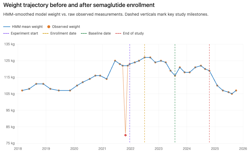
We used a method called a Hidden Markov Model (HMM). Think of it as a detective. It assumes there is a "true" weight we can't see directly, and the numbers on the chart are just noisy clues. By looking at a sequence of visits, the model weighs the clues against each other to find the most plausible underlying trajectory.

Put in slightly more technical terms, the model separates a patient’s “state” (weight at a given time) from the observations (recorded measurements) it “emits”. The state model captures gradual, coherent trajectories; the emission model accounts for noise, unit errors, and outliers. Fitted jointly across the full time series, each observation is interpreted in context — suspicious values are explained, not merely discarded. We taught the model to recognize three types of errors: normal daily fluctuations, unit mix-ups (pounds vs. kilograms), and random outliers. The result is a cleaned "trajectory" that represents what the patient likely actually weighed at each point in time.

‍

Why This Matters

When the data is cleaner, the results are more honest. We can more accurately see which treatments help patients and by how much. This ensures that the insights we share are based on what was really happening to people, not just what was typed into a computer.

The Broader Lesson

What we like about this story isn't that hidden Markov models are exotic — they're not, in the right hands. The real challenge wasn't statistical; it was domain-driven. You can't design a model that distinguishes pounds from kilograms unless someone on the team has seen that failure mode firsthand. You can't trust the trajectories unless a clinical eye confirms that's how patients on this regimen actually behave.

That cross-pollination — statisticians who think in trajectories, clinicians who think in pathways, engineers who think in pipelines — is where the creative solutions live. The unglamorous truth of working with real-world medical data is that the clever model is a byproduct. The actual value comes from having the right people willing to take the noise seriously.

‍

Technical Appendix

The HMM is composed of state transitions (the change of true weight in pounds), and of emissions (the observed weight). 

The state transitions of patient i at measurement t are given according to

where t_{it} is the difference in time passing between the two observations, we allow larger variation as the time between visits increases. The Markovian assumption becomes clear here, all information on the measurement t is provided by the observation at time t-1. 

The emissions are provided by a mixture distribution, 

where c=2.2 is the pound to kg conversion ratio. Each mixture component corresponds to a different recording mechanism. The first component represents the case where a patient’s weight is recorded in kilograms instead of pounds. The second component represents the standard case, in which the observed value is a noisy measurement of the true weight in pounds. The third component represents an outlier, modeled as a uniformly distributed value over the plausible range of observed weights. The sum of the mixing probabilities must be 1. 

Parameter Estimation

The model parameters (mixing probabilities, $$\sigma^{2}, \sigma_{\Delta}^{2} $$)  can be estimated using the expectation-maximization algorithm. EM is appropriate here because the true weight trajectory wi,t​ is unobserved, and because each recorded value may arise from one of several latent emission mechanisms: a standard pounds measurement, a kilograms-entry error, or an outlier. At a high level, the expectation step uses the current parameter values to infer the likely latent weight trajectory and to assign each observation a probability of belonging to each emission component.

The maximization step then updates the model parameters using these inferred probabilities. Observations that are likely to be standard pounds measurements contribute more strongly to the standard measurement-error component, observations likely to be kilogram entries contribute more strongly to the kilogram-entry component, and observations likely to be outliers contribute to the outlier component. The transition variability is updated from the inferred changes in true weight over time. These steps are repeated until convergence, following the standard EM framework for latent-variable models and standard HMM inference methods (Rabiner, 1989).